
Last time we talked about different levels of complexity and why engineers complicate things they complicate. And the short answer was: it’s easier that way. Not because they love to complicate things, or to prove that they can work complex things better than everyone else, but because it’s easier. It’s easier to complicate large and costly problems to make them cheaper, than trying to find massive amounts of funding needed to solve them in a simpler way. Simple is expensive.
We now know what basic erasure coding is and what it means for our storage system. But to check how it reflects in numbers, let’s brush some of our first grade math up, starting with the standard costs of writing and reading. This is our previous example:
We call this a 2+1 EC system. The data is split into 2 data chunks, 1 parity chunk is calculated, and all chunks stored at different places. Let’s assume that those different places are in fact different hosts. Distributed systems being what they are, we expect things to be distributed all over the participants anyway.
In numbers, during a 4-byte write operation, we’ll need to transfer a total of 8 bytes over the network and we’ll write 6 bytes to the physical drives - ignoring the metadata IO on the drive or packaging overhead on the network. We can actually formulate this. EC parameters are generally denoted with k and m (like k+m) so:
- Data Transferred
- = Size + Size / k x (k+m-1)
- = 4 + 4 / 2 x (2 + 1 - 1)
- = 8
- Data Written
- = Size / k x (k+m)
- = 4 / 2 x (2 + 1)
- = 6
Since we’re in first grade already:
- Data Transferred
- = Size x (2 + (m-1)/k)
- Data Written
- = Size x (1 + m/k)
In other words, EC over a distributed cluster will have small write overhead but a pretty large network overhead, in comparison to doing everything locally. See that little 2 before the data transfer factor? It means whenever you want to store some amount of data, you have to transfer at least twice that over the network first - it still wouldn’t be as high as 3x replication though. That’s why networking is so important in distributed systems. Here are some pre-calculated factors for us lazy folks:
| k | m | drive | network |
|---|---|---|---|
| 2 | 1 | 1.500 | 2.000 |
| 2 | 2 | 2.000 | 2.500 |
| 4 | 1 | 1.250 | 2.000 |
| 4 | 2 | 1.500 | 2.250 |
| 4 | 3 | 1.750 | 2.500 |
| 6 | 2 | 1.333 | 2.167 |
| 6 | 3 | 1.500 | 2.333 |
| 6 | 4 | 1.667 | 2.500 |
| 8 | 2 | 1.250 | 2.125 |
| 8 | 3 | 1.375 | 2.250 |
| 8 | 4 | 1.500 | 2.375 |
| 9 | 3 | 1.333 | 2.222 |
| 10 | 4 | 1.400 | 2.300 |
| 12 | 4 | 1.333 | 2.250 |
| 16 | 4 | 1.250 | 2.188 |
Reading is a bit simpler, if we have all the hosts running that is. In order to read 4 bytes we stored earlier, we’d need to read just those 4 bytes off the drives, meaning no extra drive overhead. Network would transfer 6 bytes total though. But in replication you’d always have the same amount of network transfer as the data because, what’s to transfer? We already have all the data we need in the first place we look for. Nevertheless the factors goes like:
| k | m | drive | network |
|---|---|---|---|
| 2 | 1 | 1.000 | 1.500 |
| 2 | 2 | 1.000 | 1.500 |
| 4 | 1 | 1.000 | 1.750 |
| 4 | 2 | 1.000 | 1.750 |
| 4 | 3 | 1.000 | 1.750 |
| 6 | 2 | 1.000 | 1.833 |
| 6 | 3 | 1.000 | 1.833 |
| 6 | 4 | 1.000 | 1.833 |
| 8 | 2 | 1.000 | 1.875 |
| 8 | 3 | 1.000 | 1.875 |
| 8 | 4 | 1.000 | 1.875 |
| 9 | 3 | 1.000 | 1.889 |
| 10 | 4 | 1.000 | 1.900 |
| 12 | 4 | 1.000 | 1.917 |
| 16 | 4 | 1.000 | 1.938 |
Using these write and read factors, we could say that it’s possible for a single write to be faster with EC but a single read will always be faster with replication. Sequential, random and/or concurrent operations are all different stories for our current level of math though.
Moving on to the ugly part: the recovery. It’s the scenario where a chunk of the data is lost and we need to re-calculate it somehow. Starting with the simple replication scenario for comparison, numbers are easy. When we lose 4 bytes in a replica, recovery is reading the same 4 bytes from a replica, sending over the network and writing them in place of the lost data. Factors are 1 for the amount of data to read from the cluster, and again 1 for the amount of data to transfer over the network.
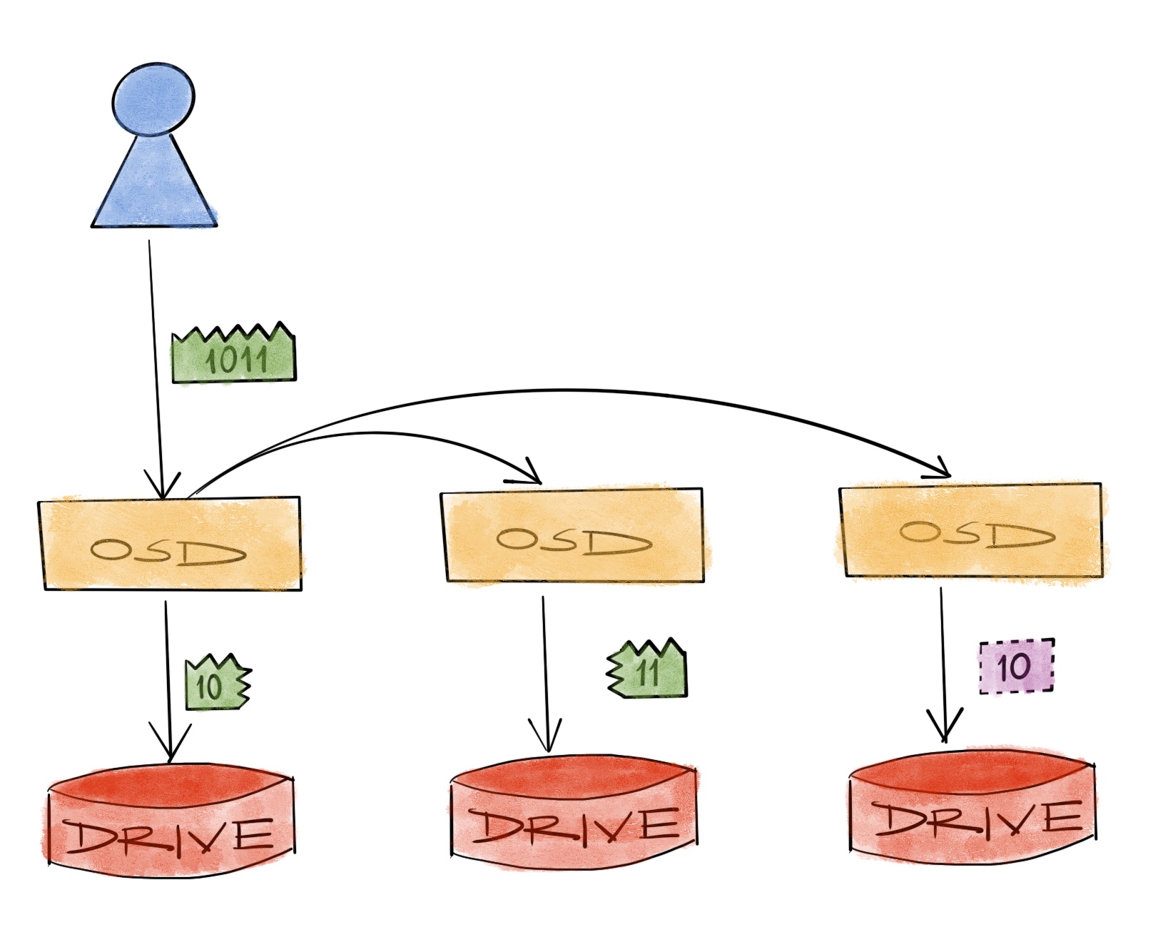
For a 2+1 EC system, when we lose a 2 byte chunk, we have to recover those 2 bytes only. But since they’re just some parts of a bigger picture and don’t have copies of them anywhere else, we need the whole picture laid down in a place to see what’s what and calculate which part we miss. So we have to read the remaining 4 bytes from the drives, transfer them over the network, find the missing 2 bytes and write them in place of the lost ones. The factors are 2 for the amount of data to read, and again 2 for the amount of data to transfer over the network.
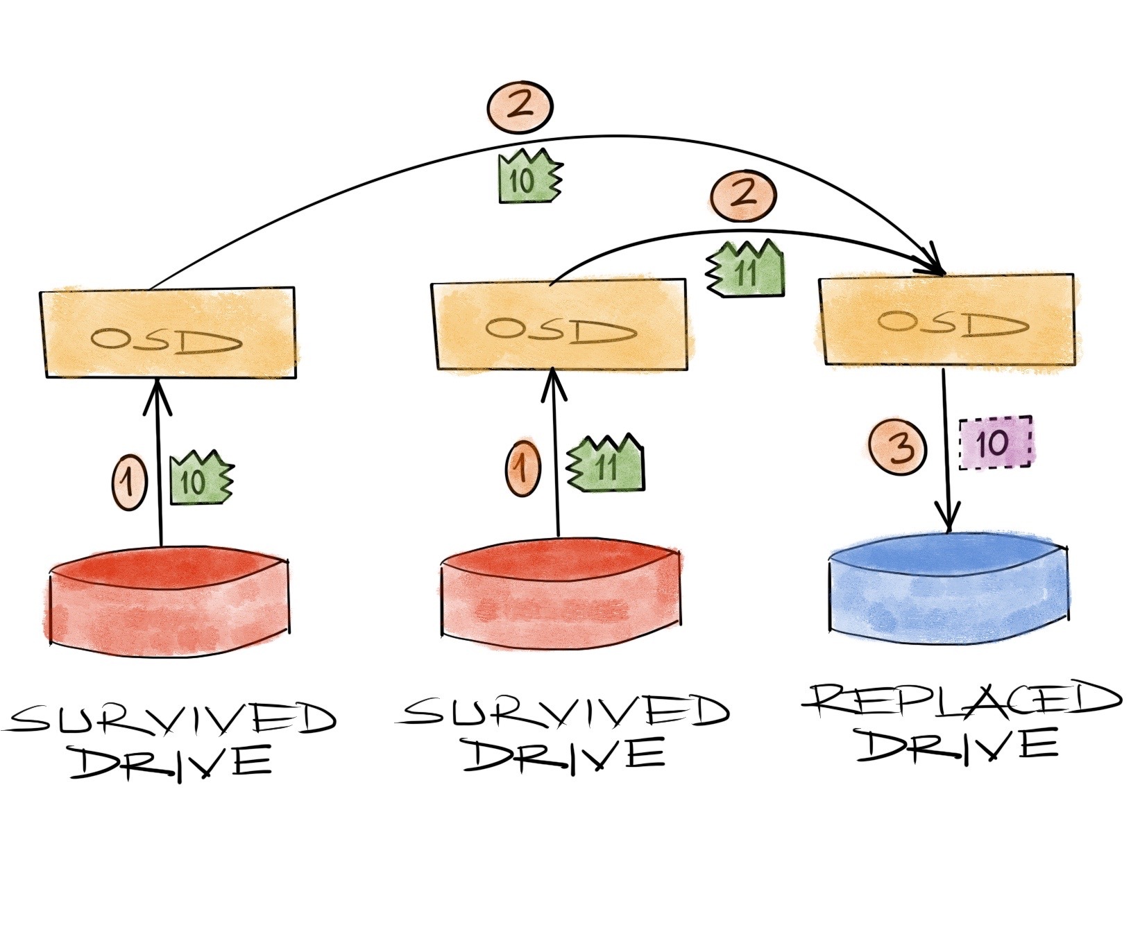
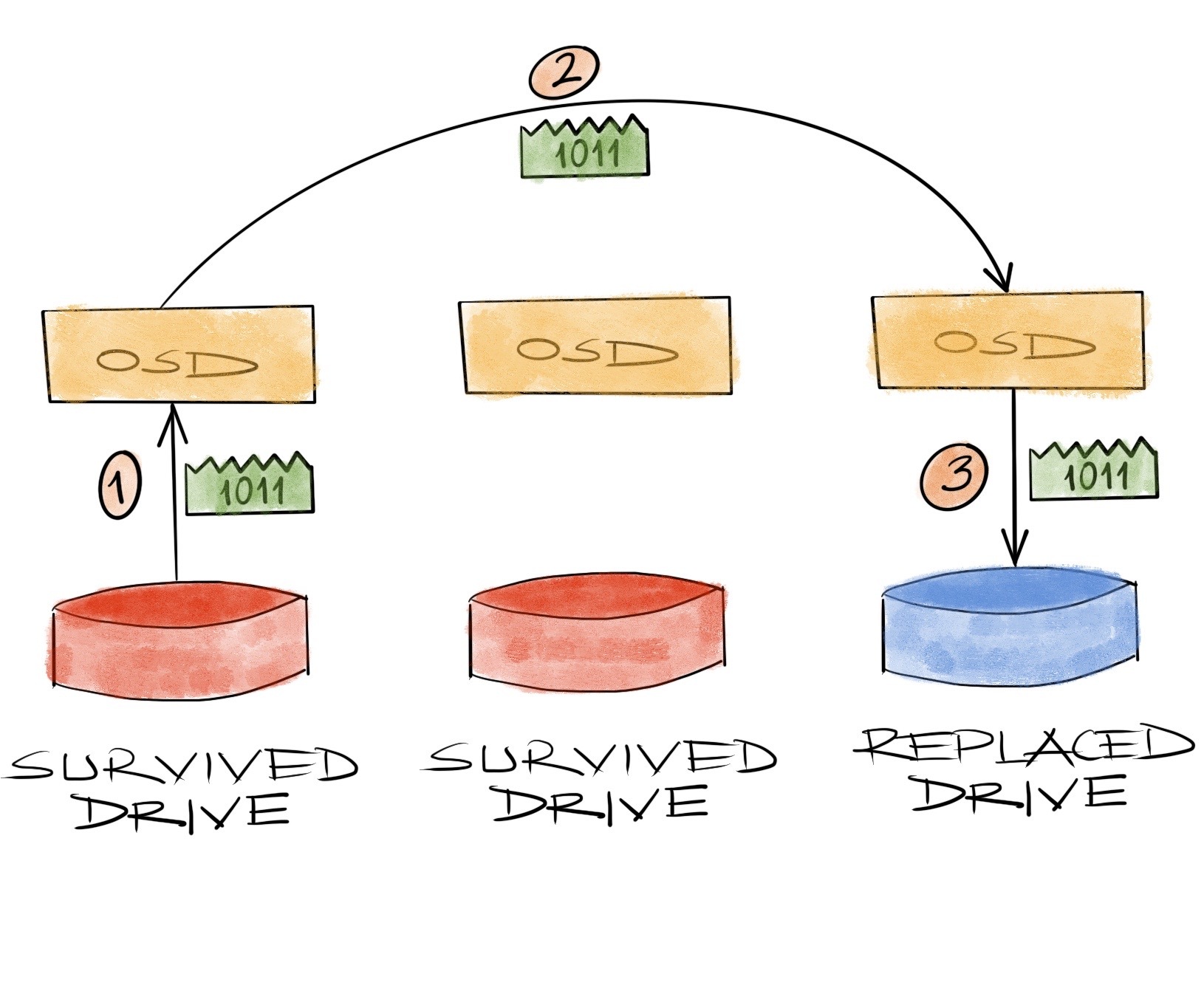
There’s a small catch in the way this is operated, though. We just assume we’re sending the remaining chunks to the place of the lost data, calculating the bytes to recover there and when we find the missing 2 bytes, we just write them to the drive. In reality, this is not how it happens in ceph. Recovery is normally run by the process on a known chunk, the primary OSD to be specific. So what happens is, the process with the known chunk collects all the remaining data from other survivors first, adds whatever it has stored in its drive, finds the missing part and transfers it to the process with the missing chunk, which only then gets written to the drive.
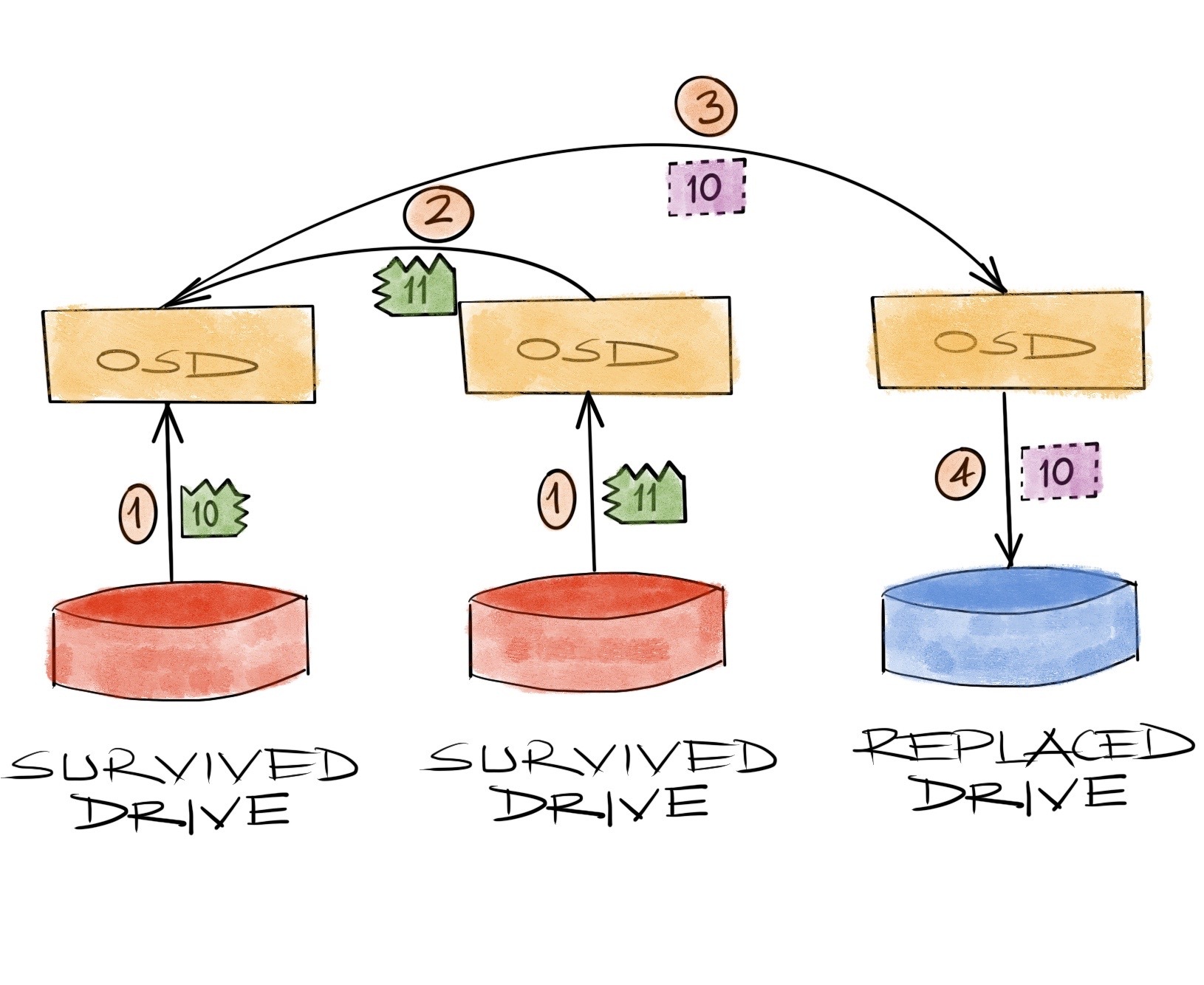
This doesn’t change the recovery network load factor, it’s still a total 2, but it affects the traffic direction. When we lose a drive and replace it, the expectation is that the data will flow from remaining hosts to the host with the replaced drive. This is a straightforward expectation in sync with our first grade logic, it’s perfectly normal. But in practice, we’ll have network traffic in and out all over our nodes.
Anyways, a factor of 2 is just 2 what’s all the fuss, right. So let’s check the factors for some other EC parameters:
| k | m | drive | network |
|---|---|---|---|
| 2 | 1 | 2 | 2 |
| 2 | 2 | 2 | 2 |
| 4 | 1 | 4 | 4 |
| 4 | 2 | 4 | 4 |
| 4 | 3 | 4 | 4 |
| 6 | 2 | 6 | 6 |
| 6 | 3 | 6 | 6 |
| 6 | 4 | 6 | 6 |
| 8 | 2 | 8 | 8 |
| 8 | 3 | 8 | 8 |
| 8 | 4 | 8 | 8 |
| 9 | 3 | 9 | 9 |
| 10 | 4 | 10 | 10 |
| 12 | 4 | 12 | 12 |
| 16 | 4 | 16 | 16 |
As you can see a 2 is not always just 2. When we need to increase our k’s and m’s because our cluster is large and we expect frequent failures, we also increase the load of the recovery on our drives and the network. See where this is going? We have a scale and cost problem on the horizon.
For example, say we design a cluster with 10 nodes. If we want to tolerate 2 simultaneous failures the m will be 2. The other parameter, k, will generally depend on our space factor requirement of say, 1.5x. This means k should be 4, so that we’ll have a 4+2 EC system and whenever we store 4 bytes we’ll end up using 6 bytes. Easy. We’ll have recovery factors 4/4 with these parameters, and since we wouldn’t have too many failures in a 10 node cluster those might be some factors we’re OK with. A standard 10G network might be plenty.
Now what if the cluster would be of 100 nodes. We might want to increase the number of simultaneous failures we’d like to tolerate to 4. And the same space factor requirement would result in EC parameters of 8+4, and recovery factors 8/8. This basically means our 10x cluster would not only have 10x nodes and hence 10x the possibility of any failure, but it also would have 2x the recovery load. Could we increase our network capacity 200x while increasing the cluster size 10x? Perhaps yes.
But perhaps, we’re not the only elementary math enthusiasts thinking about these kinds of scaling problems. These are, in fact, real problems people have in real large-scale data center environments. So coming back to the original idea, it just might be easier to complicate things. And there are indeed ways to reduce this huge network and disk load during recovery by using more complicated algorithms. Ceph supports a few different types out of the box:
- Jerasure: Reed Solomon (the default one)
- ISA: Again Reed Solomon or Cauchy, but different implementation
- LRC: Locally Repairable Erasure Code
- SHEC: Shingled Erasure Code
- CLAY: Coupled Layer
Jerasure works like the way we tried to describe up to this point. And ISA would be similar considering they’re the same algorithm. LRC, SHEC and CLAY all reduce the load during recovery in different ways. But how exactly? This would be where our teacher would tell us that she can provide us with some articles to read in our own time if we dare and we have to move on to the next lesson of “designing largish ceph clusters with capacity limits and a pretty good amount of uncertainty”. And since this post is also becoming way longer than what I expected, I’ll take this as my cue to leave it to the next one.

